GSD Calculator - Mastering Spatial Resolution for Earth Observation Satellites
At Simera Sense, we frequently experience that Ground Sampling Distance (GSD) is the main driving parameter when selecting an Earth Observation instrument, but we also see that it is maybe the least understood parameter. Determining the spatial resolution of a satellite instrument is not that straight forward and something that one cannot easily do with a GSD calculator. In this blog, we are discussing all the parameters that one should address in an ideal GSD calculator.
The next video will give you a good introduction to spatial resolution. Remember there are quite a few parameters you need to keep in mind when defining spatial resolution. Ground Sampling Distance (GSD) is only one of them.
The Limitations of a GSD Calculator
For Earth Observation instruments, we define the Ground Sampling Distance (GSD) as the geometrical separation of consecutive pixels on the ground. This distance is directly proportional to the orbital height of the satellite and the instrument’s pixel size while inversely proportional to both the focal length. The basic GSD calculator is:
GSD = Orbital Height x Pixel Size / Focal Length
Therefore, the further the satellite is from the earth and the larger the pixel size, the bigger the GSD value. A bigger GSD results in an image with less visible detail. To compensate for the bigger GSD, one can increase the focal length of the instrument; however, this results in a size increase of the payload.
As an example, a GSD of 4.75m, as the case with our MultiScape100 CIS instrument at 500 km orbital height, means that one pixel in the image represents linearly 4.75m on the ground. In practice, it means that the instrument can discriminate between objects that is 4.75m or further apart.
However, this calculation does not address the limitations of the optical system, nor the effect of diffraction.
The F-Number Impact on the GSD Calculator
Consequently, without increasing the effective optical diameter, the longer focal length translates to a higher F-number (F#). In this case, fewer photons can reach the pixels within a fixed exposure time as the “light through-put” is indirectly proportional to the F# of the system.
F# = Focal Length / Aperture Diameter
If you double the F-number, only half the number of photons can reach the focal plane. For this reason, the F# plays an essential role in determining the radiometric resolution of the optical instrument, but it is also an essential parameter to calculate the spatial cutoff frequency of the instrument and must form part of your GSD calculator.
Due to diffraction, we model an optical instrument as a low pass filter. In this case, the spatial cutoff frequency quantifies the limit beyond which the system would not be able to resolve any spatial detail. The spatial cutoff frequency is indirectly proportional to the optical wavelength (in millimetre) and F# of the system:
f0 = 1 / ( λ x F#) cycles/millimeter
As an example, when imaging at 550nm with the F6.1 optical system of the MultiScape100 CIS, the spatial cutoff frequency is 298 cycles/millimetre. For this instrument, the Nyquist Frequency of the sensor is 91 cycles/millimetre (5.5um pixel pitch). So, the optical system’s resolution limit is about three times higher than that of the high-resolution sensor. In theory, the result is sharp and crisp images.
GRD Calculator vs GSD Calculator
Ground resolved distance (GRD) relates to the diffraction-limited resolution of an optical system. The GRD calculator indicates the smallest distance that two objects can be apart for the system to be still able to distinguish between the two objects. This calculation brings the power of the optical system into the equation, something the geometric GSD calculator fails to do. The GRD is directly proportional to the orbital height and the spectral wavelength and indirectly proportional to the system’s aperture diameter:
GRD = 1.22 x Orbital Height x λ / Aperture Diameter
As an example, the MultiScape100 CIS instrument has a GRD of 3.57m at 550nm wavelength and an orbital height of 500 km. By comparing the GRD with the GSD calculation of 4.75m for the corresponding orbital height; it is evident that the optical system’s resolving power does not limit the spatial resolution.

The Modulation Transfer Function
When considering all the elements that could influence the spatial resolution of an imaging instrument, the Modulation Transfer Function (MTF) is maybe the best parameter to describe the end-to-end imaging performance. This parameter must be a fundamental part of any GSD calculator. The MTF models spatial resolution performance as a low pass filter, quantifying the amount of contrast transferred from the object to the image. The elements in the MTF model could include the atmospheric effects, the optical system limitation, the effect due to ADCS instabilities (jitter and smear) and the sensor’s constraints. As we express MTF in the frequency domain, the system MTF is a multiplication of all the underlying subsystem’s MTFs.
MTFSystem = MTFAtmosphere x MTFOptics x MTFJitter x MTFSmear x MTFSensor

Due to the scanning motion nature of an Earth ObServation satellite imager, one can always expect one-pixel smear in the along-track direction. The result is a loss of about 35% in MTF in the along-track direction. Low-frequency roll and yaw movements during the exposure time may influence the across-track MTF.
We model jitter as a Gaussian blur due to high-frequency vibrations within the structure of the satellite. Jitter has a significant impact on the MTF and must be limited to less than 10% of a pixel during a typical integration time.
Example: Sentinel-2 MTF

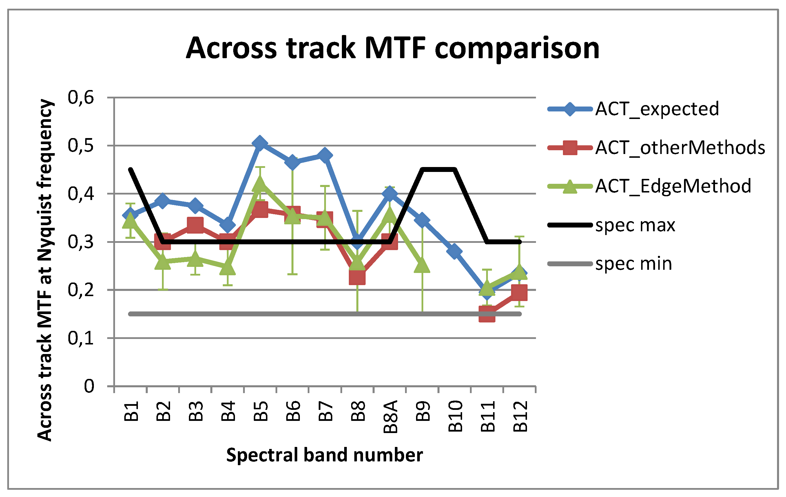
The measured Sentinel-2 Nyquist MTF values for spectral bands 2, 3, 4 in the across-track direction are between 30% and 35%. Likewise, the measured along-track values are between 20% and 30%. The GSD of these spectral bands is 10m.
The GSD Calculator: a Suite of Parameters to Consider
GSD is the most popular spatial resolution performance parameter that all new optical earth observation instrument providers are pushing. As shown in this blog, GSD is not a parameter that one could use in isolation. Other parameters to consider are GRD, the Rayleigh diffraction limit and MTF.
The single parameter that will determine the spatial resolution limits is the effective optical diameter. This parameter sets the diffraction limit of the instrument and needs to be optimised. It should also be noted that the effective optical diameter is also important when optimising the radiometric resolution.